Bringing DPPs to Language Models

These are my structured thoughts and research process in applying DPPs to language models.

Theory

The high level idea is to sample sets $S$ from an universe $\universe$ with probability $$P(S) \propto \operatorname{diversity}(S) \prod_{\yy \in S} \plm(\yy), \quad \sum_{S \subseteq \universe} P(S) = 1.$$

Distributions over sets are called sampling designs, a term that comes from survey sampling theory. They naturally model sampling without replacement.

• Given a set $\universe$ and a distribution $\plm$ over $\universe$, a sampling design is a distribution over the power set $2^\universe$ that associates each concrete subset $S \subseteq \universe$ with a probability $p(S) = \mathbb{P}(\mathcal{S} = S) \geq 0$, such that $p(S)\geq0$ and $\sum_{S \subseteq \universe} p(S) = 1$.

In simpler terms, rather than sampling one item at a time (as in i.i.d. sampling), it specifies the probability of jointly drawing a subset of items. The probability of each subset could be whatever, but it is often useful to reflect the quality of the items in the subset, i.e., $p(S) \propto \prod_{\yy \in S} p(\yy)$. Note that we are abusing notation here, as $p(\yy)$ is a different distribution over the universe, not the sampling design.

Determinantal Point Processes

• A determinantal point process (DPP) is a sampling design with the following mass function over subsets $S \subseteq \universe$: $$P_{\mathrm{DPP}}(S) \propto \det(\LL_S) \propto \operatorname{Volume}^2(\operatorname{columns}(\LL_S)),$$ where $\LL \in \mathbb{R}^{\universe \times \universe}$ is a PSD matrix, and $\LL_S$ denotes the square submatrix indexed by $S$. Efficient algorithms exist for normalization, sampling, and marginalization, but not for maximization. Computing the most likely sub-determinant is NP-hard.

• A $K$-DPP is a DPP that constrains $|S| = K$ where $K > 0$ is a parameter. $$P_{K\text{-}\mathrm{DPP}}(S) \propto \det(\LL_S)\cdot \indicator\lbrace |S| = K \rbrace.$$

Typically, we define $\LL$ with the following quality-diversity structure: $$\LL(\xx,\yy) \defeq q(\xx) \phi(\xx)^\top \phi(\yy) q(\yy),$$ where $q\colon \universe \to \mathbb{R}_{\ge 0}$ is a quality measure and $\phi\colon \universe \to \mathbb{R}^D$ a feature vector such that $\phi(\xx)^\top \phi(\yy)$ characterizes the similarity between $\xx, \yy \in \universe$. Typically, $|\phi(\xx)|_2 = 1$ and we set $q(\xx) = \sqrt{\plm(\xx)}$.

With this parametrization, the DPP mass function becomes

where abusing notation, $\phi(S) = [\phi(\xx_1), \dots, \phi(\xx_{|S|})] \in \mathbb{R}^{D \times |S|}$ is the matrix of feature vectors of the elements in $S$.

Technical details about DPPs parametrizations and sampling algorithms (for reference)

The diversity-likelihood tradeoff

If we sample from a language model using sampling techniques, we can actually draw a diversity-likelihood Pareto frontier:

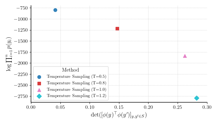
The diversity modeling is done implicitly as low temperature sampling reduces entropy, concentrating the mass on a few high-likelihood tokens. Note that applying a temperature to the step-wise softmax is not the same as applying it to the global distribution over strings.

The global K-DPP

What our parametrization of a DPP fundamentally does is to sample diverse sets from a discrete universe that has a quality measure. Ideally, we would like to define the DPP over the entire universe of possible strings $\universe = \alphabet^*$: $$\LL(\xx,\yy) = \plm(\xx) \phi(\xx)^\top \phi(\yy) \plm(\yy), \quad \LL \in \mathbb{R}^{|\universe| \times |\universe|}.$$

Of course, we cannot instantiate this matrix, which is needed to perform normalization and sampling. The following research log details our attempts to circumvent this issue.

Research log

October-November: Shah algorithm

• Idea: approximate the global DPP by iteratively instantiating a local DPP over next-token distributions. Related to Sequential Monte Carlo, Importance Sampling, Stochastic Beam Search.
• Shah & Kroese (2018) promises that any step-wise-applied set distribution converges to the global set distribution, in the sense that the final samples can be used to unbiasedly estimate expectations over the global distribution.
  • It is similar to Conditional Poisson Stochastic Beams, both do [step-wise process $\to$ global estimator], but Shah allows any set distribution.
• Problem: as in SMC, resampling induces path degeneracy. In SMC we don't care, as only one sample is produced at the end by sampling from the particle weights. However, here is crucial that we keep diversity among trajectories.
  • The algorithm is indeed diverse within last tokens, but eventually particles collapse to a common ancestor.
  • In fact, it is probable that CPSB also suffers from the same issue. Evaluating in translation tasks is very blind to path degeneracy.
  • Stochastic Beam Search does avoid path degeneracy. It explicitly models early commitment to a path, and is approximately equivalent to parallel ancestral sampling rejecting duplicates. Worth studying if it can be adapted...

December - mid January: Trying to fix Shah

• Heuristic Fix 1: Change the quality measure to be the next-token probability instead of the whole accumulated sequence probability. This way, the fact that some paths accumulate much more mass than others does not produce the degeneracy.
  • Problem: Instead of degenerating to the highest-likelihood paths, it degenerates to low-entropy paths, that concentrate mass on a few tokens.
• Heuristic Fix 2: force different paths by taking the prefix embedding $\phi(\xx[:-1])$. Now sibling nodes cannot be chosen together, as they share embedding and would cause a zero determinant to any set that includes them both.
  • No more degeneracy, but not a solution. The diversity evaluation is only using prefixes, thus the next-token selection is blind to diversity.
• Heuristic Fix 3: Intervene the local L matrices. What if we take the original formulation of the L matrix, compute the $\KK$ matrix, and then intervene it to enforce no-sibling selection while keeping the rest of the structure?
  • This is a good idea, but such intervention creates non valid $\KK$ matrices (eigenvalues outside $[0,1]$).
  • Abandoned possible fix: use semi-definite programming to find the closest valid $\KK$ matrix to the intervened one.

January-February: step-wise Shah is hard, lets first do a subpopulation-based approach

Core idea: Sample a subpopulation of $\Sigma^*$ and use it to build a DPP that approximates the global DPP. The subpopulation is $M = \lbrace \yy_1, \ldots, \yy_{|M|}\rbrace$ sampled i.i.d. from $p$ with $|M|\approx 10.000$. The naive approach is to define $\hLL$ that approximates the global $\LL$: $$\hLL(\xx,\yy) = q(\xx) \phi(\xx)^\top \phi(\yy) q(\yy), \qquad \hLL \in \mathbb{R}^{|M| \times |M|}.$$

• Problem 1: for a string $y \in S \sim DPP(\hLL(M))$ to be sampled, it must first be sampled into $M$ and then selected by the DPP. That is, $$\prob(\yy) = p(\yy \in M) p(\yy \in S \mid \yy \in M) \propto \plm(\yy)^2$$

• Problem 2: Even if we define $\hLL = \phi(M)^\top \phi(M)$ so that $\prob(\yy) \propto \plm(\yy)$, we still have to remove duplicates from $M$ to avoid zero determinants. If we do so, we are not sampling proportional to $\plm(\yy)$ anymore. To adjust for this, we can correct the $\hLL$ matrix by the probability of a string being selected at least once in the ancestral sample, i.e., $\prob(\yy \in S) = 1 - (1 - \plm(\yy))^{|M|}$. Once you do that, the approximate $\hLL$ matrix is non-PSD again 🙃.

  • TODO: are duplicates really a problem? shouldn't the DPP just ignore them?

• Alternative non-working idea: do Importance Sampling over sets. Have some other set proposal distribution and then score them with the DPP. The surprising roadblock is that despite having multiple sampling-without-replacement algorithms for LMs, which have unbiased or exact sampling algorithms and inclusion probabilities, none of them can compute $p(S)$ for a given set. A stochastic method similar to the ones employed for the inclusion probabilities should be developed. Without it, we cannot compute the importance weights.

• Solution: work with the Dual DPP. Instead of building $\hLL$ and correcting so that the end distribution is $\plm(\yy)$, estimate the $D \times D$ matrix $\CC$ using Monte Carlo. Then, sample from the Dual DPP.

  • This works! We can compute the DPP. However, it seems to sit in the Pareto frontier, not above it. 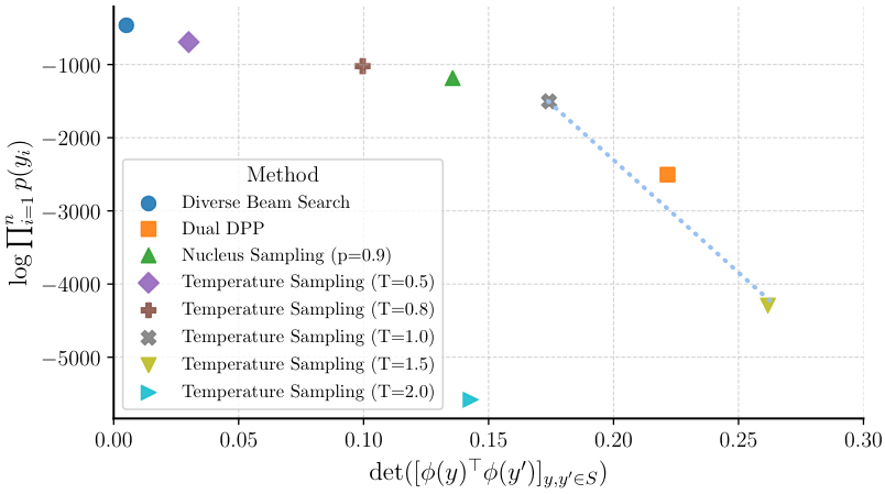The dual DPP computes more diverse sets but also less likely ones. Let's try to draw the whole frontier. How do we parametrize the Dual DPP into a curve?
  • Two ways of doing this:
    • Ryan suggests just getting a different $M$ set for each temperature, estimate a new $\CC$ matrix, and then sample from the Dual DPP.
    • Tim suggests to estimate the $\FF$ matrix using Monte Carlo, apply a temperature to the $\QQ$ matrix, and then sample from the Dual DPP.

• todo:

  • derive ancestral samples from 10k samples
  • analyze importance weights problem
  • write about the NP hardness of applying temperature to a DPP
  • write about my enhanced diversity algorithm by using an approximate DPP maximizator.